Adaptive Mesh Refinement and Coarsening

Modern supercomputers enable scientists and engineers to tackle large scale problems. However, applying a static uniform fine mesh to the whole computational domain can be extremely expensive for a grand challenge problem, and sometimes impractical.

Further, many CFD problems aim to track features that are much smaller than the overall scale of the problem, i.e., high resolutions are only required for computationally difficult regions.

An intuitive strategy to tackle this problem is to generate high-resolution meshes in needed computational regions. This strategy is the so-called adaptive mesh refinement and coarsening (AMR).

Adptivity: hp-refinement

Two types of refinement

h-refinement

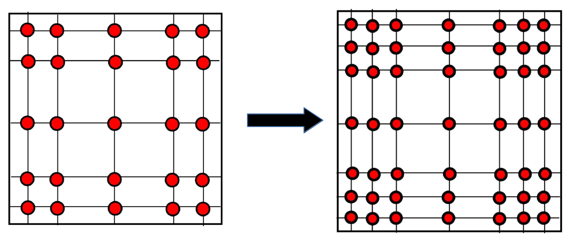
p-refinement

In this work, two types of refinement methods are invoked: h-refinement and p-refinement. h-refinement subdivides a target element into smaller children elements. p-type refinement is exclusive to high-order methods. The mesh resolution can be improved by increasing its polynomial order with respect to the target direction.

Decisions between h- and p-type refinement

A strategy to take advantage from both of the refinement methods: when the solution is poor, h-refinement should be imposed to eliminate the numerical error. Once a smooth solution is obtained, exponential convergence can be performed by prescribing p-refinement.

• Poor solution

  • h-refinement

• Smooth solution

  • p-refinement

Error Estimator

How to evaluate the smoothness of the solution?

• Use an error estimator!

An a posteriori error estimator [Mav94] is implemented in this work.

Approximated error

Approximated error = qudrature error + truncation error

\[ \begin{align}\begin{aligned}&1D: \quad \epsilon_{est} \approx \left ( \sum_{i = 0}^{N} \frac{a_i^2}{\frac{2N + 1}{2}} + \sum_{n = N+ 1}^{\infty }\frac{\widetilde{a}_n^2}{\frac{2n + 1}{2}} \right )^{1/2},\\&2D: \quad \epsilon_{est} \approx \left ( \sum_{j = 0}^{M}\frac{(a_{Nj}^2)}{\frac{2M + 1}{2}} + \sum_{i = 0}^{N}\frac{(a_{iM})^2}{\frac{2N+1}{2}} + \sum_{n = N + 1}^{\infty }\sum_{m = M + 1}^{\infty}\frac{\widetilde{a}^2_{nm}}{\frac{(2n + 1)(2m + 1)}{2^2}}\right )^{1/2}.\end{aligned}\end{align} \]

We apply a linear least squares best fit to the spectrum \(\overline{a}_n\) to get the trucation err:

\[\begin{split}\epsilon_{truc} &= \left ( \sum_{n = N + 1}^{\infty } \frac{\widetilde{a}_n^2}{\frac{2n + 1}{2}} \right )^{1/2} \\ &= \left ( \int_{N + 1}^{\infty } a_n^2 dn \right )^{1/2}\\ &= \left ( \int_{N + 1}^{\infty } \left ( Ce^{-\sigma n} \right )^2 dn \right )^{1/2} \\ &= \left ( \frac{C^2}{2\sigma } \right )^{1/2}e^{-\sigma (N + 1)},\end{split}\]

where \(\sigma\) can be seen as an error indicator. It describes the decay rate of the local truncation error.

Refinement Criteria

When to refine?

The refinement criterion is simple: refine the element when its estimated error \(\epsilon_{est}\) exceeds the threshold:

\[\epsilon_{est} \geq \epsilon u_h,\]

where \(\epsilon\) is the discretization tolerance and \(u_h\) is the approximated solution.

h-type or p-type of refinement?

• \(\sigma > 1\) --> good local resolution. --> p-refinement.

• \(\sigma \leq 1\) --> poor local resolution. --> h-refinement.

Coarsening?

Coarsening is applied when the estimated error is smaller than the defined smallest tolerance, \(\epsilon_{min}\):

\[\epsilon_{est} \leq \epsilon_{min} \left \| u_h \right \|.\]

The error estimator makes good use of the feature of the local polynomial spectrum, which makes it work independently of the system of equations being solved.